• PyTorch
• Tensors
  • 1D Tensor
  • 2D Tensor
  • 3D Tensor
• Linear Regression Model

PyTorch

PyTorch is a scalable and multiplatform programming interface for implementing and running machine learning algorithms. PyTorch is primarily developed at Facebook AI Research lab. Many machine learning researchers and practitioners from academia and industry have adapted PyTorch to develop deep learning solutions, such as Tesla Autopilot, Uber’s Pyro, and Hugging Face’s Transformers.

Tensors

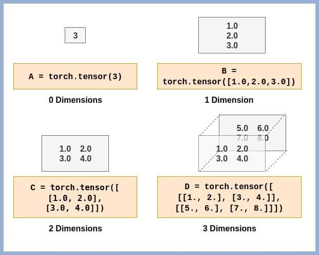
Tensors are the fundamentals data structures used in machine learning, in context of data science tensors are multi-dimensional arrays of numbers that represent complex data.

1D Tensor

import torch
import numpy as np

# Create a 1D tensor (vector)
tensor_1d = torch.tensor([1, 2, 3, 4, 5])
print(tensor_1d)

tensor([1, 2, 3, 4, 5])

2D Tensor

# Create a 2D tensor (matrix)
tensor_2d = torch.tensor([[1, 2, 3], [4, 5, 6], [7, 8, 9]])
print(tensor_2d)

tensor([[1, 2, 3], [4, 5, 6], [7, 8, 9]])

3D Tensor

tensor_3d = torch.tensor([[[1, 2, 3], [4, 5, 6]],
                          [[7, 8, 9], [10, 11, 12]]])

tensor([[[ 1, 2, 3], [ 4, 5, 6]], [[ 7, 8, 9], [10, 11, 12]]])

Linear Regression Model

At its core, linear regression seeks to establish a linear relationship between a dependent variable (often denoted as ( y )) and one or more independent variables (denoted as ( x )). The simplest form, simple linear regression, involves a single independent variable and is represented by the equation:

where:

• \(( y )\) is the dependent variable.
• \(( x )\) is the independent variable.
• \(( \beta_0 )\) is the y-intercept of the regression line.
• \(( \beta_1 )\) is the slope of the regression line.
• \(( \epsilon )\) is the error term, accounting for the variability in ( y ) that ( x ) cannot explain.

In multiple linear regression, the model extends to include multiple independent variables, and the equation becomes:

where:

• \(( y )\) is the dependent variable.
• \(( x_1, x_2, \ldots, x_n )\) are the independent variables.
• \(( \beta_0 \ )\) is the y-intercept of the regression plane.
• \(( \beta_1, \beta_2, \ldots, \beta_n )\) are the coefficients representing the impact of each independent variable.
• \(( \epsilon )\) is the error term.

The goal of linear regression is to determine the optimal values of \(( \beta_0, \beta_1, \ldots, \beta_n )\) that minimize the sum of squared differences between the observed values and the values predicted by the model, known as the residual sum of squares (RSS). This optimization is typically performed using methods such as Ordinary Least Squares (OLS).

Linear regression provides a straightforward yet powerful approach to predictive modeling, making it a cornerstone technique in the field of data science.

import torch
import numpy as np
import matplotlib.pyplot as plt

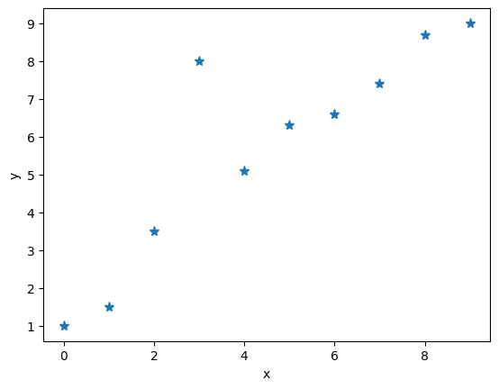
X_train = np.arange(10, dtype="float32").reshape((10, 1))
y_train = np.array([1.0, 1.5, 3.5, 8, 5.1,
                    6.3, 6.6,7.4, 8.7, 9.0])

plt.plot(X_train, y_train, '*', markersize=8)
plt.xlabel("x")
plt.ylabel("y")
plt.show()

we will standardize the features (mean centering and dividing by the standard deviation)

from torch.utils.data import TensorDataset
from torch.utils.data import DataLoader

X_train_norm = (X_train - np.mean(X_train)) / np.std(X_train)
X_train_norm = torch.from_numpy(X_train_norm)
y_train = torch.from_numpy(y_train)
train_ds = TensorDataset(X_train_norm, y_train)
batch_size = 1
train_dl = DataLoader(train_ds, batch_size, shuffle=True)

Now, we can define our model for linear regression as $z = wx + b$. Here we will use the torch.nn module as it provides predefined layer for building complex NN models and use stochastic gradient descent as the optimizer from torch.optim modules.

torch.manual_seed(1)
weight = torch.randn(1)
weight.requies_grad_()
bias = torch.zeros(1, requies_grad=True)

Here we initialized weight and bias vector. After defining the model we need to define loss function that we want to minimize to find optimal weight. We will choose mean squared error (MSE) as our loss function.

loss_fn = nn.MSELoss(reduction='mean')
input_size, output_size = 1, 1
learning_rate = 0.01
num_epochs = 200

model = nn.Linear(input_size, output_size)
optimizer = torch.optim.SGD(model.parameters(), lr=learning_rate)

Note, we used torch.nn.Linear class for linear layer to perform $z = wx + b$ calculation. Now, we can call step() method of the optimizer to train the model and pass batched dataset we created above.

for epoch in range(num_epochs):
    for x_batch, y_batch in train_dl:
        # 1. Generate predictions
        pred = model(x_batch)[:, 0]

        # 2. Calculate loss
        loss = loss_fn(pred, y_batch)

        # 3. Compute gradients
        loss.backward()

        # 4. Update parameters using gradients
        optimizer.step()

        # 5. Reset the gradients to zero
        optimizer.zero_grad()

    if epoch % log_epochs==0:
        print(f'Epoch {epoch} Loss {loss.item():.4f}')

After the model is trained we can check the weight and bias parameters

print("Final Paremeters:", model.weight.item(), model.bias.item())

Final Paremeters: 2.419365882873535 5.718400955200195

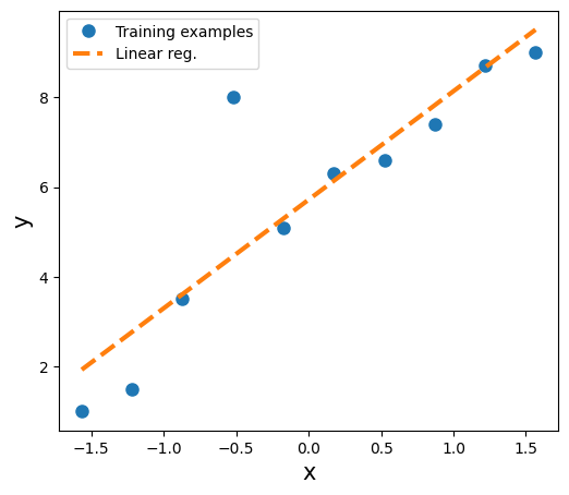
For the test data, we created NumPy array of values evenly spaced between 0 and 9 and apply the same standardization features as the train dataset.

# Test data
X_test = np.linspace(0, 9, num=100, dtype='float32').reshape(-1, 1)
X_test_norm = (X_test - np.mean(X_train)) / np.std(X_train)
X_test_norm = torch.from_numpy(X_test_norm)

# Prediction
y_pred = model(X_test_norm).detach().numpy()

# Plot
fig = plt.figure(figsize=(13, 5))
ax = fig.add_subplot(1, 2, 1)
plt.plot(X_train_norm, y_train, 'o', markersize=8)
plt.plot(X_test_norm, y_pred, '--', lw=3)
plt.legend(['Training examples', 'Linear reg.'])
ax.set_xlabel('x', size=15)
ax.set_ylabel('y', size=15)
ax.tick_params(axis='both', which='major')
plt.show()