System Modeling in Flexsim
Introduction:
FlexSim, a cutting-edge simulation software, has revolutionized the way businesses approach process optimization and efficiency enhancement. Throughout my journey of learning and understanding FlexSim, I embarked on an exciting project that allowed me to explore the vast capabilities of this powerful tool. In this blog, I will provide a detailed layout of the FlexSim project I undertook, shedding light on my learning process, key challenges faced, and the valuable insights gained along the way.
Project Overview:
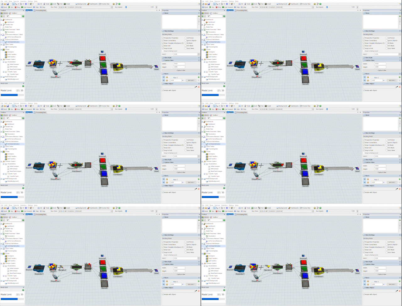
In this project, I built a simple simulation model using FlexSim to gain hands-on experience with its components and functionalities. The model incorporated fixed resources, task executor objects, port connections, statistical distributions, labels, triggers, and data analysis through the pin dashboard feature. By simulating a basic system, I explored the behavior and efficiency of the simulated system, introduced variability through statistical distributions, and tracked relevant information using labels. The use of triggers, combiner objects, and dispatcher objects allowed for dynamic control, while the pin dashboard provided visual representations for data analysis. Through this project, I developed a solid foundation in FlexSim, equipping myself with valuable skills for future simulation modeling endeavors in process optimization and efficiency enhancement.
Model Development:
Considering the constraint of 30 models in the student version of FlexSim, I focused on building a small yet insightful simulation model. The model consists of a fixed resource source that generates flow items, which then pass through a separator object. The separator object randomly outputs items with a specified quantity using the dunifrom distribution. To add more variation, I included a trigger in the separator object to label and color the items upon exit. This resulted in different colored boxes representing the exiting items, with an empirical distribution assigned to each item using weights.
The flow items then proceed to a queue and subsequently to a downstream processor. In the downstream processor, I utilized the lognormalmeanstdev distribution to set the process time for each item. Notably, each item was assigned its own mean and standard deviation using a global table, enabling individualized processing times based on specific characteristics.
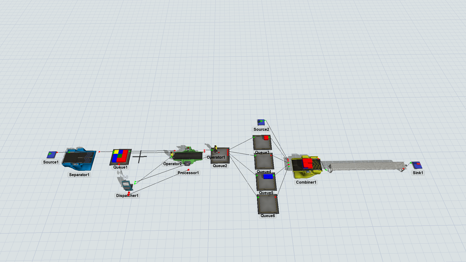
Following the downstream processor, the flow items proceed to another queue before being distributed to four separate queues based on their item types. Each queue represents a specific category of items within the simulation model. From the four queues, the items flow into a combiner belt, where a pallet from a source object combines the items together. This step simulates the process of assembling or packaging multiple items into a single unit.
After the items are combined on the combiner belt, they continue to flow onto a conveyor belt. The conveyor belt serves as a means of transporting the combined items to their final destination. Finally, the items reach the sink object, which represents the end of the process or system being simulated. The sink object collects the items, signifying their completion or removal from the simulation model.
Through this series of steps involving queues, combiner belts, conveyor belts, and a sink object, the simulation model replicates a process in which flow items are collected, combined, transported, and ultimately reach their final destination.
By implementing this flow path within the simulation model, I gained hands-on experience in modeling system with multiple components and processes. This allowed me to explore the dynamics of item flow, queue management, and the overall efficiency of the simulated process.
Results:
After simulateing the model, I utilized various visual tools to showcase the outcomes of the simulation model built in FlexSim. By generating graphs, I was able to effectively analyze and present behavior of the simulated system.
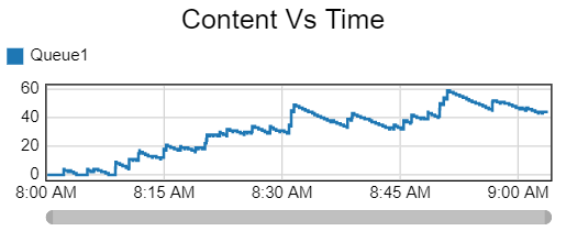
The graphs created provided valuable insights into key metrics such as throughput staytime, and much more advanced graphs can be create to analyze the system. These graphs allows to identify bottlenecks, and evaluate the overall efficiency of the simulated process. By analyzing the data represented in the graphs, we can make informed observations and draw conclusions regarding system performance and potential areas for improvement.
Below are some other graphs that I created to further analyze and visualize the results of the simulation model

In FlexSim, “State” represents the current condition of an entity, while “Staytime” refers to the time an entity remains in a specific location. State helps track entity progress, while Staytime controls entity duration in a process or location.
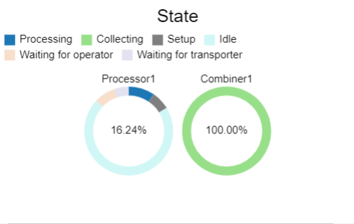
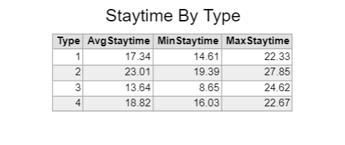
Overall, a comprehensive analysis of the simulation model’s performance and behavior using bar charts, line charts box plot, Gantt Chart etc. By combining quantitative data with visual representations, we can effectively communicate the insights gained from the simulation runs. These results serve as a valuable resource for further analysis, decision-making, and potential optimization efforts in real-world scenarios.
Despite the model’s simplicity, it provides a valuable learning opportunity by incorporating various distribution types, triggers, labels, and dynamic attributes. Through this model, I gained practical experience in utilizing statistical distributions, global tables, and object properties to simulate real-world scenarios. This foundation will prove beneficial as I progress to more complex simulation projects in the future.
